X

Real Numbers

Euclid’s Division Lemma

Given positive integers \(a\) and \(b\), there exist unique integers \(q\) and \(r\) satisfying \(a = bq + r\), \(0 \leq r < b\).

Euclid’s division algorithm, as the name suggests, has to do with divisibility of integers. Stated simply, it says any positive integer \(a\) can be divided by another positive integer \(b\) in such a way that it leaves a remainder \(r\) that is smaller than \(b\).

Let us see how the algorithm works, through an example first. Suppose we need to find the HCF of the integers \(455\) and \(42\). We start with the larger integer, that is, \(455\). Then we use Euclid’s lemma to get

\(455 = 42 \times 10 + 35\)

Now consider the divisor \(42\) and the remainder \(35\), and apply the division lemma to get

\(42 = 35 \times 1 + 7\)

Now consider the divisor \(35\) and the remainder \(7\), and apply the division lemma to get

\(35 = 7 \times 5 + 0\)

Notice that the remainder has become zero, and we cannot proceed any further. We claim that the HCF of \(455\) and \(42\) is the divisor at this stage, i.e., \(7\).

Every positive even integer is of the form \(2q\), and every positive odd integer is of the form \(2q + 1\), where \(q\) is some integer.

The Fundamental Theorem of Arithmetic

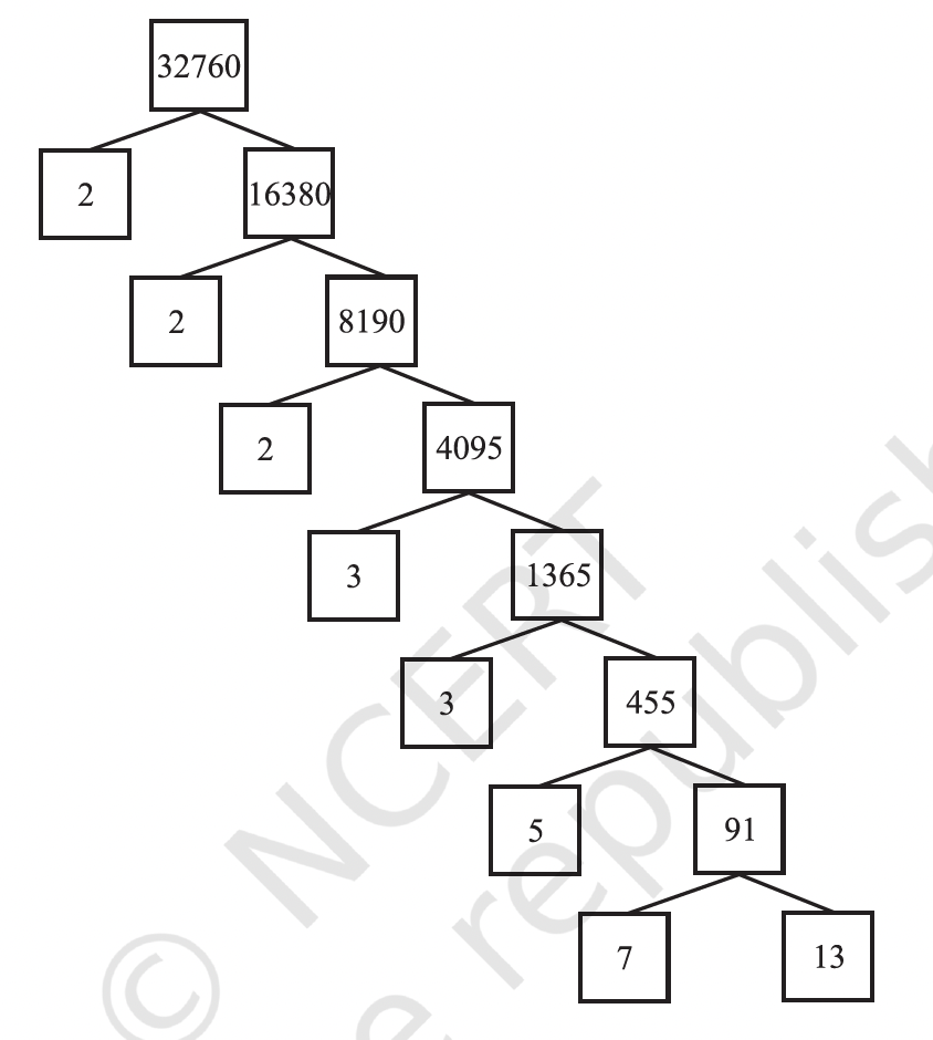
Every composite number can be expressed ( factorised) as a product of primes, and this factorisation is unique, apart from the order in which the prime factors occur.

Any natural number can be written as a product of its prime factors. For instance, \(2 = 2\), \(4 = 2 \times 2\), \(253 = 11 \times 23\)

Note

A composite number is a natural number (a positive whole number greater than 1) that has more than two factors (divisors) i.e. \(1\) and itself.

Note that \(\text{HCF}(6, 20) = 2^1 = \text{Product of the smallest power of each common}\) prime factor in the numbers.

\(\text{LCM}(6, 20) = 2^2 \times 3^1 \times 5^1 = \text{Product of the greatest power of each prime factor}\), involved in the numbers.

From the example above, you might have noticed that \(\text{HCF}(6, 20) \times \text{LCM}(6, 20) = 6 \times 20\).

In fact, we can verify that for any two positive integers \(a\) and \(b\), \(\text{HCF}(a, b) \times \text{LCM}(a, b) = a \times b\).

The key to understanding this lies in the prime factorization of the two numbers, \(a\) and \(b\).

Let’s say the prime factorization of \(a\) and \(b\) are as follows:

\(a = p_1^{a_1} \times p_2^{a_2} \times \dots \times p_n^{a_n}\) \(b = p_1^{b_1} \times p_2^{b_2} \times \dots \times p_n^{b_n}\)

where \(p_1, p_2, \dots, p_n\) are all the prime factors that appear in either \(a\) or \(b\) (or both), and \(a_i\) and \(b_i\) are non-negative integers representing the exponents of these prime factors in the factorization of \(a\) and \(b\), respectively. If a prime factor doesn’t appear in a number’s factorization, its exponent is 0.

Now, let’s think about how we find the HCF and LCM using these prime factorizations:

• Highest Common Factor (HCF): The HCF is the product of the common prime factors raised to the lowest power they appear in either factorization. \(\text{HCF}(a, b) = p_1^{\min(a_1, b_1)} \times p_2^{\min(a_2, b_2)} \times \dots \times p_n^{\min(a_n, b_n)}\)

• Least Common Multiple (LCM): The LCM is the product of all the prime factors that appear in either factorization raised to the highest power they appear in either factorization. \(\text{LCM}(a, b) = p_1^{\max(a_1, b_1)} \times p_2^{\max(a_2, b_2)} \times \dots \times p_n^{\max(a_n, b_n)}\)

Now, let’s consider the product of the HCF and the LCM:

\(\text{HCF}(a, b) \times \text{LCM}(a, b) = (p_1^{\min(a_1, b_1)} \times p_2^{\min(a_2, b_2)} \times \dots \times p_n^{\min(a_n, b_n)}) \times (p_1^{\max(a_1, b_1)} \times p_2^{\max(a_2, b_2)} \times \dots \times p_n^{\max(a_n, b_n)})\)

We can rearrange this product by grouping the powers of the same prime factors together:

\(\text{HCF}(a, b) \times \text{LCM}(a, b) = p_1^{\min(a_1, b_1) + \max(a_1, b_1)} \times p_2^{\min(a_2, b_2) + \max(a_2, b_2)} \times \dots \times p_n^{\min(a_n, b_n) + \max(a_n, b_n)}\)

Now, here’s the crucial insight: for any two numbers \(x\) and \(y\), the sum of their minimum and maximum is equal to their sum:

\(\min(x, y) + \max(x, y) = x + y\)

Applying this to the exponents of our prime factors:

\(\min(a_i, b_i) + \max(a_i, b_i) = a_i + b_i\)

So, our product becomes:

\(\text{HCF}(a, b) \times \text{LCM}(a, b) = p_1^{a_1 + b_1} \times p_2^{a_2 + b_2} \times \dots \times p_n^{a_n + b_n}\)

We can rewrite this using the properties of exponents:

\(\text{HCF}(a, b) \times \text{LCM}(a, b) = (p_1^{a_1} \times p_2^{a_2} \times \dots \times p_n^{a_n}) \times (p_1^{b_1} \times p_2^{b_2} \times \dots \times p_n^{b_n})\)

And recognizing the original prime factorizations of \(a\) and \(b\):

\(\text{HCF}(a, b) \times \text{LCM}(a, b) = a \times b\)

In simpler terms, the logic is this:

When you find the HCF, you take the common prime factors with their smallest exponents. When you find the LCM, you take all the prime factors with their largest exponents.

When you multiply the HCF and the LCM together, for each prime factor, you’re essentially combining the smallest and largest exponent from the original numbers. This combination reconstructs the original exponents of that prime factor in both \(a\) and \(b\) when multiplied together.

Let’s take our example of 6 and 20 again:

\(6 = 2^1 \times 3^1\) \(20 = 2^2 \times 5^1\)

HCF(6, 20) = \(2^{\min(1, 2)} \times 3^{\min(1, 0)} \times 5^{\min(0, 1)} = 2^1 \times 3^0 \times 5^0 = 2 \times 1 \times 1 = 2\) LCM(6, 20) = \(2^{\max(1, 2)} \times 3^{\max(1, 0)} \times 5^{\max(0, 1)} = 2^2 \times 3^1 \times 5^1 = 4 \times 3 \times 5 = 60\)

Now, let’s multiply the HCF and LCM:

HCF \(\times\) LCM = \(2 \times 60 = 120\)

And let’s multiply the original numbers:

\(6 \times 20 = 120\)

As you can see, they are equal!

Polynomials

Let’s break down the key features of a polynomial: term, coefficient, variable, exponent, and degree.

1. Term:

• A term in a polynomial is a product of a constant (the coefficient) and one or more variables raised to non-negative integer powers.

• Terms are separated by addition (+) or subtraction (-) signs.

  • Examples: In the polynomial \(3x^2 - 5x + 7\), the terms are \(3x^2\), \(-5x\), and \(7\).

2. Coefficient:

• The coefficient of a term is the numerical factor that multiplies the variable part of the term.

  • Examples:

    • In the term \(3x^2\), the coefficient is 3.

    • In the term \(-5x\), the coefficient is -5.

    • In the term \(7\) (which can be thought of as \(7x^0\)), the coefficient is 7.

    • If a term is just a variable like \(y\), its coefficient is understood to be 1 (since \(1y = y\)).

3. Variable:

• A variable is a symbol (usually a letter like \(x\), \(y\), \(z\), etc.) that represents an unknown or changing value.

• Polynomials can have one or more variables.

  • Examples:

    • \(2x + 1\) (one variable: \(x\))

    • \(x^2y - 3xy + 4y^2\) (two variables: \(x\) and \(y\))

4. Exponent (or Power):

• The exponent (or power) of a variable in a term indicates how many times the variable is multiplied by itself.

• For an expression to be a polynomial, the exponents of the variables in each term must be non-negative integers (0, 1, 2, 3, …).

  • Examples:

    • In the term \(3x^2\), the exponent of \(x\) is 2.

    • In the term \(-5x\) (which is \(-5x^1\)), the exponent of \(x\) is 1.

    • In the term \(7\) (which is \(7x^0\)), the exponent of \(x\) is 0.

  • Not polynomial terms:

    • \(x^{-1}\) (negative exponent)

    • \(\sqrt{x}\) or \(x^{1/2}\) (fractional exponent)

    • \(\frac{1}{x}\) (variable in the denominator, equivalent to \(x^{-1}\))

5. Degree:

The concept of degree can be applied to both individual terms and the entire polynomial:

• Degree of a Term:

  • For a term with one variable, the degree is simply the exponent of that variable.

    • Example: The degree of \(3x^2\) is 2. The degree of \(-5x\) is 1. The degree of \(7\) is 0.

  • For a term with more than one variable, the degree is the sum of the exponents of all the variables in that term.

    • Example: The degree of \(2x^3y^2\) is \(3 + 2 = 5\). The degree of \(-4xy^4\) is \(1 + 4 = 5\). The degree of \(6ab\) (which is \(6a^1b^1\)) is \(1 + 1 = 2\).

• Degree of a Polynomial:

  • The degree of a polynomial is the highest degree of any of its terms with a non-zero coefficient.

  • Examples:

    • The degree of \(3x^2 - 5x + 7\) is 2 (because the term with the highest degree is \(3x^2\), which has a degree of 2).

    • The degree of \(x^3y - 2xy^2 + 5\) is 3 (because the term with the highest degree is \(x^3y\), which has a degree of \(3+1=4\)? No, \(x^3y\) has degree \(3+1=4\). Let’s re-evaluate. The degree of \(x^3y\) is \(3+1=4\). The degree of \(-2xy^2\) is \(1+2=3\). The degree of \(5\) is \(0\). So the degree of the polynomial is 4).

    • The degree of \(7y + 2\) is 1 (linear polynomial).

    • The degree of \(15\) is 0 (constant polynomial).

A polynomial of degree 1 is called a linear polynomial. For example, \(2x - 3\), \(\sqrt{3}x + 5\), \(y + 2\), \(\frac{11}{2}x\), \(3z + 4\), \(\frac{1}{3}u\), etc., are all linear polynomials.

A polynomial of degree 2 is called a quadratic polynomial. For example, \(x^2 + 3x + 2\), \(2x^2 - 3x + 1\), \(3x^2 + 4\), \(5x^2 - 6x + 7\), \(8y^2 + 9y + 10\), etc., are all quadratic polynomials.

A polynomial of degree 3 is called a cubic polynomial. For example, \(x^3 + 2x^2 + 3x + 4\), \(2x^3 - 3x^2 + 4\), \(5x^3 - 6x^2 + 7x + 8\), \(9y^3 + 10y^2 + 11y + 12\), etc., are all cubic polynomials.

Zeroes of a Polynomial

If \(p(x)\) is a polynomial in \(x\), and if \(k\) is any real number, then the value obtained by replacing \(x\) by \(k\) in \(p(x)\), is called the value of \(p(x)\) at \(x = k\), and is denoted by \(p(k)\).

In general, if \(k\) is a zero of \(p(x) = ax + b\), then \(p(k) = ak + b = 0\), i.e., \(k = -\frac{b}{a}\)

So, the zero of the linear polynomial \(ax + b\) is \(\frac{-b}{a}\) = \(\frac{-(Constant term)}{Coefficient of x}\).

Geometrical meaning of the Zeroes of a Polynomial

import matplotlib.pyplot as plt
import numpy as np

x = np.linspace(-100,100)

fig, ax = plt.subplots()
ax.plot(x,(2*x + 3))

ax.text(1,1.6,'$y = 2x+3$')

ax.set_xlim(-8,8)
ax.set_ylim(-8,8)
ax.axvline(color='k',linewidth = 1)
ax.axhline(color='k',linewidth = 1)

ax.set_xticks(list(range(-8,8)))
ax.set_aspect('equal')
ax.grid(True,ls=':')

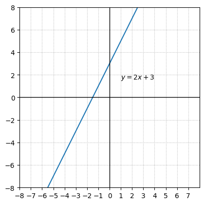
Geometrically, the zero of a linear polynomial is the x-coordinate of the point where the graph of the polynomial intersects the x-axis. Since a linear polynomial represents a straight line, it will intersect the x-axis at exactly one point. For a linear polynomial in the form of \(ax + b\), the zero is \((-b/a,0)\), which is where the line crosses the x-axis.

Geometrical meaning of a zero of a quadratic polynomial

x = np.linspace(-50,50,1000)

fig, ax = plt.subplots()
ax.plot(x,(x**2 - 3*x - 4))

ax.text(1,1.6,'$y = x^2 -3x - 4$')

ax.set_xlim(-8,8)
ax.set_ylim(-8,8)
ax.axvline(color='k',linewidth = 1)
ax.axhline(color='k',linewidth = 1)

ax.set_xticks(list(range(-8,8)))
ax.set_aspect('equal')
ax.grid(True,ls=':')

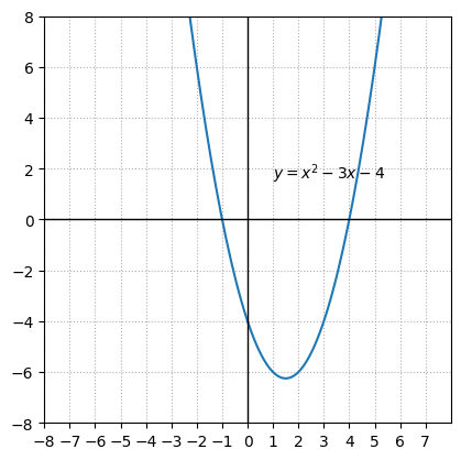
In fact, for any quadratic polynomial \(ax^2 + bx + c\), where \(a \neq 0\), the graph of the corresponding equation \(y = ax^2 + bx + c\) has one of two shapes:

• opens upwards when \(a > 0\)

• opens downwards when \(a < 0\) (These curves are called parabolas.)

Geometrically, the zeroes of a quadratic polynomial \(ax^2 + bx + c\) (where \(a \neq 0\)) are the x-coordinates of the points where the graph of the polynomial, which is a parabola (\(y = ax^2 + bx + c\)), intersects the x-axis.

Here’s a breakdown of the possibilities:

• Two distinct zeroes: The parabola intersects the x-axis at two different points. The x-coordinates of these two points are the two distinct zeroes of the quadratic polynomial.

• One zero (two equal zeroes): The parabola touches the x-axis at exactly one point (the vertex of the parabola lies on the x-axis). In this case, the quadratic polynomial has one zero, which is considered a repeated root or two equal zeroes.

• No real zeroes: The parabola does not intersect or touch the x-axis at any point. In this case, the quadratic polynomial has no real zeroes. The zeroes are complex numbers.

In summary, the number of real zeroes of a quadratic polynomial corresponds to the number of times its graph intersects the x-axis. A quadratic polynomial can have at most two real zeroes.

Discriminant

The discriminant of a quadratic equation of the form \(ax^2 + bx + c = 0\) (where \(a\), \(b\), and \(c\) are real numbers and \(a \neq 0\)) is a value that helps determine the nature of the roots (or zeroes) of the equation. It is denoted by the Greek letter delta (\(\Delta\)) and is calculated using the formula:

\(\Delta = b^2 - 4ac\)

The value of the discriminant tells us three crucial things about the roots:

1. If \(\Delta > 0\) (\(b^2 - 4ac > 0\)):

   • The quadratic equation has two distinct real roots.

   • Geometrically, the graph of \(y = ax^2 + bx + c\) intersects the x-axis at two different points.

2. If \(\Delta = 0\) (\(b^2 - 4ac = 0\)):

   • The quadratic equation has one real root (a repeated or double root).

   • Geometrically, the vertex of the graph of \(y = ax^2 + bx + c\) touches the x-axis at exactly one point.

3. If \(\Delta < 0\) (\(b^2 - 4ac < 0\)):

   • The quadratic equation has no real roots. The roots are a pair of complex conjugate numbers.

   • Geometrically, the graph of \(y = ax^2 + bx + c\) does not intersect the x-axis. It lies entirely above or entirely below the x-axis.

Why is it called the discriminant?

The term “discriminant” is used because it discriminates or distinguishes between the different types of roots a quadratic equation can have based on the values of its coefficients.

Connection to the Quadratic Formula:

The discriminant appears under the square root sign in the quadratic formula, which gives the roots of the equation:

\(x = \frac{-b \pm \sqrt{b^2 - 4ac}}{2a} = \frac{-b \pm \sqrt{\Delta}}{2a}\)

• If \(\Delta > 0\), \(\sqrt{\Delta}\) is a real, non-zero number, leading to two different real solutions (\(-b + \sqrt{\Delta})/(2a)\) and \((-b - \sqrt{\Delta})/(2a)\).

• If \(\Delta = 0\), \(\sqrt{\Delta} = 0\), leading to one real solution \(x = -b/(2a)\).

• If \(\Delta < 0\), \(\sqrt{\Delta}\) is an imaginary number, leading to two complex conjugate solutions.

In summary, the discriminant is a powerful tool for quickly understanding the nature of the roots of a quadratic equation without fully solving it.

Note

In general, given a polynomial \(p(x)\) of degree \(n\), the graph of \(y = p(x)\) intersects the x-axis at at most \(n\) points. Therefore, a polynomial \(p(x)\) of degree \(n\) has at most \(n\) zeroes. Zeroes or roots of a polynomial are the values of \(x\) for which \(p(x) = 0\).

Pair of Linear Equations in Two Variables

Each solution \((x, y)\) of a linear equation in two variables, \(ax + by + c = 0\), corresponds to a point on the line representing the equation, and vice versa.

Types of Pairs of Linear Equations:

• Inconsistent pair: These equations have no solution. Geometrically, this means the lines represented by the equations are parallel and never intersect.

• Consistent pair: These equations have at least one solution. This category is further divided:

  • Unique solution: The lines intersect at a single point.

  • Infinitely many solutions (Dependent pair): The lines are coincident, meaning they are essentially the same line. Every point on the line is a common solution.

Geometric Interpretation and Algebraic Conditions:

Algebraic conditions based on the coefficients of the linear equations in the standard form:

\(a_1x + b_1y = c_1\) \(a_2x + b_2y = c_2\)

• (i) Intersecting Lines (Unique Solution - Consistent): The condition for intersecting lines is: \(\frac{a_1}{a_2} \neq \frac{b_1}{b_2}\)

• (ii) Coincident Lines (Infinitely Many Solutions - Dependent & Consistent): The condition for coincident lines is: \(\frac{a_1}{a_2} = \frac{b_1}{b_2} = \frac{c_1}{c_2}\)

• (iii) Parallel Lines (No Solution - Inconsistent): The condition for parallel lines is: \(\frac{a_1}{a_2} = \frac{b_1}{b_2} \neq \frac{c_1}{c_2}\)

This is a fundamental concept in algebra when dealing with systems of linear equations. It allows you to predict the nature of the solution(s) without actually solving the system.

Arithmetic Progression

An arithmetic progression is a list of numbers in which each term is obtained by adding a fixed number to the preceding term except the first term. This fixed number is called the common difference of the AP. Remember that it can be positive, negative or zero

The \(n\) th term \(a_n\) of an AP with first term \(a\) and common difference \(d\) is given by \(a_n = a + (n - 1)d\).

The sum of the first \(n\) terms of an AP is given by \(S_n = \frac{n}{2}(a + l)\), where \(a\) is the first term and \(l\) is the last term.