Linear Algebra#
Vectors#
import numpy as np
import matplotlib.pyplot as plt
A vector is a one-dimensional matrix.
The size of the vectors is determined by its rows or how many numbers it has.
For example, \(\mathbf{x}\) is \(3\times 1\) meaning it has 3 rows and 1 column.
Vectors in numpy#
# alternatively you can perform x[:,np.newaxis]
x = np.array([1,2,3]).reshape(-1,1)
print('column vector in numpy: \n',x)
print('Shape of the vector is ',x.shape)
column vector in numpy:
 [[1]
 [2]
 [3]]
Shape of the vector is  (3, 1)
Vectors in coordinate plane#
Vectors that are \(2\times 1\) are said to belong to \(\mathbb{R}^2\), meaning that they belong to
the set of real numbers that come paired two at a time. The capital \(\mathbb{R}\) is used
to emphasize that you’re looking at real numbers. You also say that \(2\times 1\)
vectors, or vectors in \(\mathbb{R}^2\), are a part of two-space.
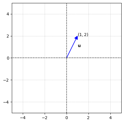
Vectors in 2 space are represented on the coordiante \((x,y)\) plane by rays. In standard position, the ray representing a vector has its endpoint at the origin and its terminal point (or arrow) at the \((x,y)\) coordinates designated by the column vector. The \(x\) coordinate is in the first row of the vector, and the \(y\) coordinate is in the second row.
Here \(\mathbf{u}\) \(\in\) \(\mathbb{R}^2\), and can be represented in the \((x,y)\) plane as \((1,2)\).
fig, ax = plt.subplots()
options = {"head_width":0.3, "head_length":0.3, "length_includes_head":True}

u = np.array([1,2]).reshape(-1,1)

ax.arrow(0,0,u[0][0],u[1][0],fc='b',ec='b',**options)

ax.text(1,1,'$\mathbf{u}$')
ax.text(1,2,'$(1,2)$')

# settings
ax.set_aspect('equal')
ax.grid(True,ls=':')
ax.axvline(x=0,color="k",ls=":")
ax.axhline(y=0,color="k",ls=":")
ax.grid(True)
ax.axis([-5,5,-5,5])
ax.set_aspect('equal')
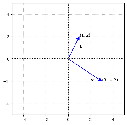
We can add another vector,
where \(\mathbf{v}\) \(\in\) \(\mathbb{R}^2\), and can be represented in the \((x,y)\) plane as \((3,-2)\).
fig, ax = plt.subplots()
options = {"head_width":0.3, "head_length":0.3, "length_includes_head":True}

v = np.array([3,-2]).reshape(-1,1)

ax.arrow(0,0,u[0][0],u[1][0],fc='b',ec='b',**options)
ax.arrow(0,0,v[0][0],v[1][0],fc='b',ec='b',**options)

ax.text(1,1,'$\mathbf{u}$')
ax.text(1,2,'$(1,2)$')
ax.text(2,-2,'$\mathbf{v}$')
ax.text(3,-2,'$(3,-2)$')

# settings
ax.set_aspect('equal')
ax.grid(True,ls=':')
ax.axvline(x=0,color="k",ls=":")
ax.axhline(y=0,color="k",ls=":")
ax.grid(True)
ax.axis([-5,5,-5,5])
ax.set_aspect('equal')
You aren’t limited to always drawing \(2\times 1\) vectors radiating from the origin. Both the vectors drawn above can start from \((-1,2)\) as an endpoint.
fig, ax = plt.subplots()
options = {"head_width":0.3, "head_length":0.3, "length_includes_head":True}

ax.arrow(-1,2,u[0][0],u[1][0],fc='b',ec='b',**options)
ax.arrow(-1,2,v[0][0],v[1][0],fc='b',ec='b',**options)

ax.text(-4,1,'$endpoint (-1,2)$')
ax.text(-1.5,3,'$\mathbf{u}$')
ax.text(0,4,'$(0,4)$')
ax.text(1,1,'$\mathbf{v}$')
ax.text(2,0,'$(2,0)$')

# settings
ax.set_aspect('equal')
ax.grid(True,ls=':')
ax.axvline(x=0,color="k",ls=":")
ax.axhline(y=0,color="k",ls=":")
ax.grid(True)
ax.axis([-6,6,-6,6])
ax.set_aspect('equal')
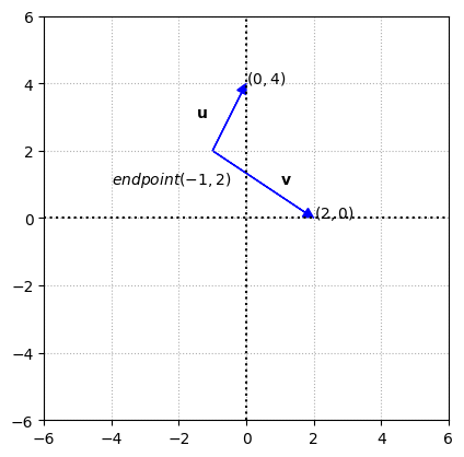
Notice that the vectors have the same lengths and point in the same direction with the same slant. What we did above, is simply moving \(x\) or \(y\) steps away from the endpoint. In other words, we simply add the \(\mathbf{u}\) with the \(endpoint\) vector to get a resulting vector
which is the terminal point \((0,4)\). We shall look at computations on vectors in detail.
Vectors can actually have many number of rows, although its difficult to illustrate vectors that have more than 3 rows, which implies 3 spaces.
For example,
where \(\mathbf{w}\) \(\in\) \(\mathbb{R}^3\), and can be represented in the \((x,y,z)\) plane as \((2,3,4)\). Three-space vectors are represented by three-dimensional figures and arrows pointing to positions in space.
The different geometric transformations performed on vectors include rotations, reflections, expansions, and contractions.
Scalar multiplication#
When you multiply a \(2\times 1\) vector by a scalar, your result is another \(2\times 1\) vector. A scalar is a real number — a constant value. Multiplying a vector by a scalar means that you multiply each element in the vector by the same constant value.
where we multiply the vector \(\mathbf{v}\) by \(scalar\) \(k\). Below is an example
Vectors have operations that cause dilations (expansions) and contractions (shrinkages) of the original vector. Both operations of dilation and contraction are accomplished by multiplying the elements in the vector by a scalar.
If the scalar, k, that is multiplying a vector is greater than 1, then the result is a dilation of the original vector. If the scalar, k, is a number between 0 and 1, then the result is a contraction of the original vector.
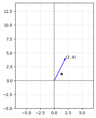
For example, consider a vector \(\mathbb{a}\)
multiplying it with a scalar say 3 will result in dilation or expansion and with \(\frac{1}{2}\) results in contraction or shrinking.
fig, ax = plt.subplots()
options = {"head_width":0.3, "head_length":0.3, "length_includes_head":True}

a = np.array([2,4]).reshape(-1,1)

ax.arrow(0,0,a[0][0],a[1][0],fc='b',ec='b',**options)

ax.text(1,1,'$\mathbf{a}$')
ax.text(2,4,'$(2,4)$')
# settings
ax.set_aspect('equal')
ax.grid(True,ls=':')
ax.axvline(x=0,color="k",ls=":")
ax.axhline(y=0,color="k",ls=":")
ax.grid(True)
ax.axis([-7,7,-5,14])
ax.set_aspect('equal')
fig, ax = plt.subplots(1,3, figsize=(15, 15))
options = {"head_width":0.3, "head_length":0.3, "length_includes_head":True}

for i,scl in enumerate([1,3,0.5]):
    a_d = (scl * a).astype(int)
    ax[i].arrow(0,0,a_d[0][0],a_d[1][0],fc='b',ec='b',**options)
    ax[i].text(a_d[0][0],a_d[1][0],f'$({a_d[0][0]},{a_d[1][0]})$')
    # settings
    ax[i].set_aspect('equal')
    ax[i].grid(True,ls=':')
    ax[i].axvline(x=0,color="k",ls=":")
    ax[i].axhline(y=0,color="k",ls=":")
    ax[i].grid(True)
    ax[i].axis([-9,9,-5,14])
    ax[i].set_aspect('equal')
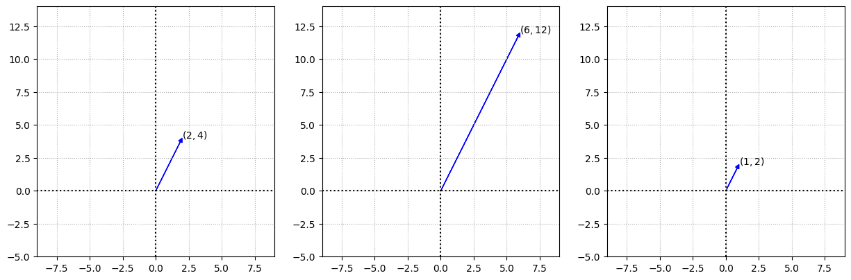
As you can see, the length of the vector is affected by the scalar multiplication, but the direction or angle with the axis (slant) is not changed.
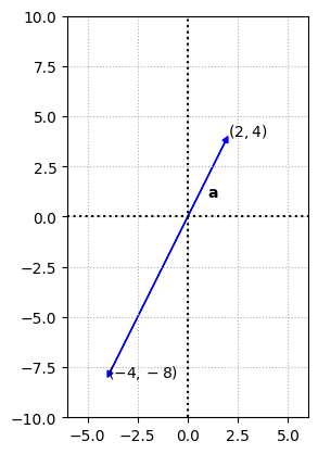
When multiplying a vector by a negative scalar, these things happen:
The size of the vector changes i.e. each element in the vector changes and has a greater absolute value (except with –1).
The direction of the vector reverses.
Multiplying vector \(\mathbb{a}\) with -2 will give
fig, ax = plt.subplots()
options = {"head_width":0.3, "head_length":0.3, "length_includes_head":True}

a_d = -2 * a

ax.arrow(0,0,a[0][0],a[1][0],fc='b',ec='b',**options)
ax.arrow(0,0,a_d[0][0],a_d[1][0],fc='b',ec='b',**options)

ax.text(1,1,'$\mathbf{a}$')
ax.text(2,4,'$(2,4)$')
ax.text(-4,-8,'$(-4,-8)$')

# settings
ax.set_aspect('equal')
ax.grid(True,ls=':')
ax.axvline(x=0,color="k",ls=":")
ax.axhline(y=0,color="k",ls=":")
ax.grid(True)
ax.axis([-6,6,-10,10])
ax.set_aspect('equal')
Vector addition and subtraction#
The vectors have to be of the same size to add one another or subtract from one another. This process involves adding or subtracting the corresponding elements in the vectors like a one-to-one match up.
For example
We can illustrate what is happening when we add 2 vectors. For example
fig, ax = plt.subplots()
options = {"head_width":0.3, "head_length":0.3, "length_includes_head":True}

u = np.array([2,4]).reshape(-1,1)
v = np.array([3,1]).reshape(-1,1)
u_v = u + v

ax.arrow(0,0,u[0][0],u[1][0],fc='b',ec='b',**options)
ax.arrow(u[0][0],u[1][0],v[0][0],v[1][0],fc='b',ec='b',**options)
ax.arrow(0,0,u_v[0][0],u_v[1][0],fc='b',ec='k',**options)

ax.text(-1,2,'$(2,4)$')
ax.text(2,5,'$(3,1)$')
ax.text(5,5,'$(5,5)$')

# settings
ax.set_aspect('equal')
ax.grid(True,ls=':')
ax.axvline(x=0,color="k",ls=":")
ax.axhline(y=0,color="k",ls=":")
ax.grid(True)
ax.axis([-8,8,-10,10])
ax.set_aspect('equal')

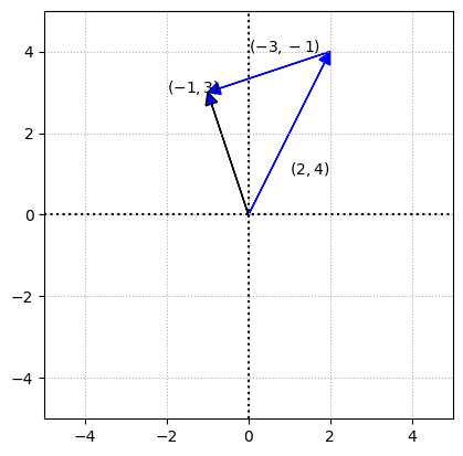
we are adding the second vector to the terminal point of the first vector, result is the vector obtained from vector addition.
Vector subtraction is just another way of saying that you’re adding one vector to a second vector that’s been multiplied by the scalar –1. For example
fig, ax = plt.subplots()
options = {"head_width":0.3, "head_length":0.3, "length_includes_head":True}

v = -1 * v
u_v = u + v

ax.arrow(0,0,u[0][0],u[1][0],fc='b',ec='b',**options)
ax.arrow(u[0][0],u[1][0],v[0][0],v[1][0],fc='b',ec='b',**options)
ax.arrow(0,0,u_v[0][0],u_v[1][0],fc='b',ec='k',**options)

ax.text(1,1,'$(2,4)$')
ax.text(0,4,'$(-3,-1)$')
ax.text(-2,3,'$(-1,3)$')

# settings
ax.set_aspect('equal')
ax.grid(True,ls=':')
ax.axvline(x=0,color="k",ls=":")
ax.axhline(y=0,color="k",ls=":")
ax.grid(True)
ax.axis([-5,5,-5,5])
ax.set_aspect('equal')
Vector magnitude#
The magnitude of a vector is also referred to as its length or norm. It is the length of the ray that you see in two-space or three-space. Vectors with more
than three rows also have magnitude, and the computation is the same although its not possible to visually picture it.
The magnitude of \(\mathbb{v}\) is denoted by \(\lVert \mathbb{v} \rVert\). The formula is
where \(v_1^2, v_2^2, v_3^2, \dots ,v_n^2\) are the elements of the vector.
When you multiply a vector by a scalar, then the magnitude is also multiplied, i.e. \(\lvert k \rvert \cdot \lVert \mathbb{v} \rVert\). For example
then the magnitude is
By multiplying the vector with 3 results in
which is simply 3 times the actual magnitude. Although in the case of negative scalar consider the absolute value.
Triangle inequality#
The magnitude of the sum of vectors is always less than or equal to the sum of the magnitudes of the vectors.
from numpy import linalg as LA

u = np.array([23,10,18]).reshape(-1,1)
# alternatively mag_u = np.sqrt(np.sum(np.square(u)))
mag_u = LA.norm(u)
v = np.array([1,4,12]).reshape(-1,1)
mag_v = LA.norm(v)
u_v = u + v
mag_uv = LA.norm(u_v)

print('u = \n',u,'\n magnitude:', mag_u)
print('v = \n',v,'\n magnitude:', mag_v)
print('u + v = \n', u_v,'\n magnitude:', mag_uv)
u =
 [[23]
 [10]
 [18]]
 magnitude: 30.870698080866262
v =
 [[ 1]
 [ 4]
 [12]]
 magnitude: 12.68857754044952
u + v =
 [[24]
 [14]
 [30]]
 magnitude: 40.890096600521744
Inner product#
The inner product of two real valued vectors is also called the dot product. When \(u\) and \(v\) are both \(n × 1\) vectors, then the notation \(u^Tv\) indicates the inner product of \(u\) and \(v\).
The dot product is calculated as the sum of the products of corresponding elements of two vectors, hence to change its orientation we transpose \(u\). The superscript \(T\) in the notation means to transpose.
u = np.array([1, -2, 1, 4]).reshape(-1,1)
v = np.array([2, -3, 9, 5]).reshape(-1,1)
u = np.array([1, -2, 1, 4]).reshape(-1,1)
v = np.array([2, -3, 9, 5]).reshape(-1,1)
# alternatively you can just use a 1d array and use numpy dot
# i.e. uv_dot = np.dot(u.transpose(),v)
uv_dot = np.vdot(u,v)

print('u = \n', u)
print('v = \n', v)
print('Dot product:', uv_dot)
u =
 [[ 1]
 [-2]
 [ 1]
 [ 4]]
v =
 [[ 2]
 [-3]
 [ 9]
 [ 5]]
Dot product: 37
We shall explore these topics in detail when working with matrices in later sections.
Orthoganality#
The slope of a line is determined by finding the difference between the y-coordinates of two points on the line and dividing that difference by the difference between the corresponding x-coordinates of the points on that line.
To determine whether two lines are perpendicular to each other, you can compare their slopes. Their slopes are negative reciprocals. That is
or
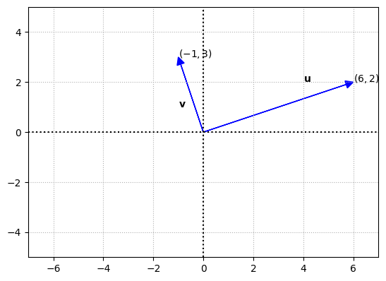
Two lines, segments, or planes are said to be orthogonal if they’re perpendicular to one another.
When dealing with vectors, if the inner product is equal to 0, then the vectors are perpendicular.
u = np.array([6,2]).reshape(-1,1)
v = np.array([-1,3]).reshape(-1,1)

uv_dot = np.vdot(u,v)

print('u = \n', u)
print('v = \n', v)
print('Dot product:', uv_dot)

y = np.array([u[1][0],0])
x = np.array([u[0][0],0])
# we use the function gradient from numpy to find change in y with respect to x
u_slope = np.gradient(y, x)

y = np.array([v[1][0],0])
x = np.array([v[0][0],0])
v_slope = np.gradient(y, x)

print('slope of u = ', u_slope[0])
print('slope of v = ', v_slope[0])
print('product of the slopes = ', u_slope[0] * v_slope[0])

fig, ax = plt.subplots()
options = {"head_width":0.3, "head_length":0.3, "length_includes_head":True}

ax.arrow(0,0,u[0][0],u[1][0],fc='b',ec='b',**options)
ax.arrow(0,0,v[0][0],v[1][0],fc='b',ec='b',**options)

ax.text(4,2,'$\mathbf{u}$')
ax.text(u[0][0],u[1][0],'$(6,2)$')
ax.text(-1,1,'$\mathbf{v}$')
ax.text(v[0][0],v[1][0],'$(-1,3)$')

# settings
ax.set_aspect('equal')
ax.grid(True,ls=':')
ax.axvline(x=0,color="k",ls=":")
ax.axhline(y=0,color="k",ls=":")
ax.grid(True)
ax.axis([-7,7,-5,5])
ax.set_aspect('equal')
u =
 [[6]
 [2]]
v =
 [[-1]
 [ 3]]
Dot product: 0
slope of u =  0.3333333333333333
slope of v =  -3.0
product of the slopes =  -1.0
Angle between two vectors#
There is a relation between the inner product, magnitude and the angle between two vectors.
where \(u\) and \(v\) are two vectors in two-space, \(u \cdot v\) is the inner product of the two vectors, \(\lVert u \rVert\) and \(\lVert v \rVert\) are the respective magnitudes of the vectors, and \(cos \theta\) is the measure (counterclockwise) of the angle formed between the two vectors.
So to determine the angle \(\theta\)
So for the graph above, since the vectors are perpendicular to each other, the angle formed is 90°. We can also confirm this by performing the computation using the relation described.
uv_dot = np.vdot(u,v)
mag_u = LA.norm(u)
mag_v = LA.norm(v)

cos_theta = uv_dot / mag_u * mag_v

# compute the angle in radians
theta_radians = np.arccos(cos_theta)
# convert radians to degrees
theta_degrees = np.degrees(theta_radians)

print("Dot product of u and v =", uv_dot)
print("Magnitude of u =", mag_u)
print("Magnitude of v =", mag_v)
print("cos theta =", cos_theta)
print("Angle in radians =", theta_radians)
print("Radians to degrees =",theta_degrees)
Dot product of u and v = 0
Magnitude of u = 6.324555320336759
Magnitude of v = 3.1622776601683795
cos theta = 0.0
Angle in radians = 1.5707963267948966
Radians to degrees = 90.0
Matrices#
A matrix is made up of rows and columns surrounded by a bracket. You have same number of elements in each row and same number of elements in each column.
Matrices are defined by a capital letter. The elements are named with lowercase letters with subscripts (index of the element). For example, \(a_{13}\) in a matrix corresponds to the element in row 1 and column 3 of \(A\) i.e. 3. So the general notion for the elements in a matrix \(A\) is \(a_{ij}\).
The dimension of the matrix \(A\) is \(3 \times 3\), which means that it has 3 rows and 3 columns.
Adding and subtracting#
To add or subtract two matrices, the dimension of the matrices must be the same. You simply add or subtract the corresponding element in the matrices. Let \(A\) and \(B\) be two \(m \times n\) matrices. Then
Matrix addition is commutative. However, matrix subtraction is not commutative.
\(A + B = B + A\)
\(A-B \ne B - A\)
# creation of a matrix in numpy
A = np.matrix([[1, 2, 3], [4, 5, 6], [7,8,9]])
# Alternative to create a matrix from 1d array
A_arr = np.array([1, 2, 3,4, 5, 6, 7,8,9])
A = np.matrix(A_arr.reshape(3,3))
# create another matrix
B = np.matrix(A_arr.reshape(3,3))

print("A = \n",A)
print("The dimension of A = ", A.shape)
print("B = \n",B)
print("The dimension of B = ", B.shape)
print('A + B = \n', A + B)
A =
 [[1 2 3]
 [4 5 6]
 [7 8 9]]
The dimension of A =  (3, 3)
B =
 [[1 2 3]
 [4 5 6]
 [7 8 9]]
The dimension of B =  (3, 3)
A + B =
 [[ 2  4  6]
 [ 8 10 12]
 [14 16 18]]
Matrix multiplication#
Multiplying a matrix \(A\) with a scalar \(k\) implies multiplying every element in the matrix with the scalar.
k = 2
kA = k * A

print("k =", 2)
print("kA = \n", kA)
k = 2
kA =
 [[ 2  4  6]
 [ 8 10 12]
 [14 16 18]]
To perform matrix multiplication on two matrices, the number of columns in the first matrix should be equal to the number of rows in the second matrix. If \(A\) is \(m \times n\) matrix and \(B\) is \(p \times q\) matrix, then it is necessary that \(n = p\). The dimension of the resulting matrix is a \(m \times q\).
For example, if \(A\) has dimension \(3 \times 4\) and \(B\) has dimension \(4 \times 7\), then the product \(A * B\) has dimension \(3 \times 7\). But you can’t multiply the matrices in the reverse order. The product \(B * A\) cannot be performed, because \(B\) has seven columns and \(A\) has three rows.
Each element in the new matrix created by matrix multiplication is the sum of all the products of the elements in a row of the first matrix times a column in the second matrix.
\(X\) is a \(2 \times 3\) matrix. \(Y\) is a \(3 \times 4\) matrix. Since the number of columns in \(X\) is the same as the number of rows in \(Y\), then \(X * Y\) is
where \(a_{12}\) is found by multiplying the elements in the first row of \(X\) by the elements in the second column of \(Y\) i.e. 1(2) + (2)(6) + (3)(10) = 44.
X = np.matrix(np.arange(1,7,1).reshape(2,3))
Y = np.matrix(np.arange(1,13,1).reshape(3,4))
# alternatively you can create 2d numpy arrays and use @ instead of * to perform matrix multiplication
XY = X * Y

print('X = \n', X)
print('Y = \n', Y)
print('X * Y = \n', XY)
X =
 [[1 2 3]
 [4 5 6]]
Y =
 [[ 1  2  3  4]
 [ 5  6  7  8]
 [ 9 10 11 12]]
X * Y =
 [[ 38  44  50  56]
 [ 83  98 113 128]]
Matrix multiplication is not commutative. Even if the condition for rows and columns satisfy, the product is not the same when the matrices are reversed. If \(C\) and \(D\) are square matrices of dimension \(3 \times 3\), then \(C * D \ne D * C\).
There are special cases where matrix multiplication is commutative:
When multiplying by the multiplicative identity on a square matrix
When multiplying by the inverse of the matrix — if the matrix does, indeed, have an inverse.
We shall look at this in later sections.
Identity matrix#
The additive identity in arithmetic is 0. If you add 0 to a number, you don’t change the number — the number keeps its identity. The multiplicative identity in arithmetic is 1.
The additive identity for matrices is the \(zero\) matrix. The additive identity for a \(3 \times 4\) matrix is a \(3 \times 4\) zero matrix. If
then the \(zero\) matrix is
The multiplicative identity is a square matrix and the elements on the main diagonal running from the top left to the bottom right are 1s. All the rest of the elements in the matrix are 0s.
If \(D\) is a \(3 \times 2\) matrix, when multiplying \(D * I\) where \(I\) is the identity matrix, then \(I\) has to be a \(2 \times 2\) matrix where the main diagonals has 1s and all the other elements are 0s. When multiplying \(I * D\) then \(I\) is a \(3 \times 3\) matrix.
Earlier we inferred that the multiplication of matrices is not commutative. The special case is when a \(square\) matrix is multiplied by its identity matrix.
import numpy.matlib

D = np.arange(1,7).reshape(3,2)
# alternatively you can use numpy eye or identity function that creates a 2d array of identity matrix
I = np.matlib.identity(D.shape[1])

DI = D @ I

print("D = \n", D)
print("I = \n", I)
print("D * I = \n", DI)

I = np.matlib.identity(D.shape[0])

ID = I @ D

print("I = \n", I)
print("I * D = \n", ID)
D =
 [[1 2]
 [3 4]
 [5 6]]
I =
 [[1. 0.]
 [0. 1.]]
D * I =
 [[1. 2.]
 [3. 4.]
 [5. 6.]]
I =
 [[1. 0. 0.]
 [0. 1. 0.]
 [0. 0. 1.]]
I * D =
 [[1. 2.]
 [3. 4.]
 [5. 6.]]
Triangular and diagonal matrices#
Triangular and diagonal matrices are square matrices. \(A\) is an upper triangular matrix, because all the elements below the main diagonal are 0s. \(B\) is a lower triangular matrix, because all the elements above the main diagonal are 0s. \(C\) is diagonal matrix, because all the elements above and below the main diagonal are 0s.
Singular and non-singular matrices#
Two numbers are multiplicative inverses if their product is 1 (the multiplicative identity). For example, 4 and 1/4 are multiplicative inverses. When a matrix has a multiplicative inverse, the product of the matrix and its inverse is equal to an identity matrix (multiplicative identity).
A square matrix is singular if it has a multiplicative inverse; a matrix is non-singular if it does not have a multiplicative inverse.
Properties under addition#
Matrix addition is commutative; if you add \(A\) to \(B\), you get the same result as adding \(B\) to \(A\).
A = np.matrix(np.arange(1,10).reshape(3,3))
B = A * 2

AB = A + B
BA = B + A

print('A = \n', A)
print('B = \n', B)
print('A + B = \n', AB)
print('B + A = \n', BA)
print('A + B == B + A is', np.array_equal(AB,BA))
A =
 [[1 2 3]
 [4 5 6]
 [7 8 9]]
B =
 [[ 2  4  6]
 [ 8 10 12]
 [14 16 18]]
A + B =
 [[ 3  6  9]
 [12 15 18]
 [21 24 27]]
B + A =
 [[ 3  6  9]
 [12 15 18]
 [21 24 27]]
A + B == B + A is True
Matrix addition is associative.
A = np.matrix(np.arange(1,10).reshape(3,3))
B = A * 2
C = B + 2

AB = A + B
AB_C = AB + C
BC = B + C
BC_A = BC + A

print('A = \n', A)
print('B = \n', B)
print('C = \n', C)
print('(A + B) + C = \n', AB_C)
print('A + (B + C) = \n', BC_A)
print('(A + B) + C == A + (B + C) is', np.array_equal(AB_C,BC_A))
A =
 [[1 2 3]
 [4 5 6]
 [7 8 9]]
B =
 [[ 2  4  6]
 [ 8 10 12]
 [14 16 18]]
C =
 [[ 4  6  8]
 [10 12 14]
 [16 18 20]]
(A + B) + C =
 [[ 7 12 17]
 [22 27 32]
 [37 42 47]]
A + (B + C) =
 [[ 7 12 17]
 [22 27 32]
 [37 42 47]]
(A + B) + C == A + (B + C) is True
Properties under multiplication#
Matrix multiplication, as a rule, is not commutative. The exceptions involve multiplying a matrix by its inverse or by the multiplicative identity.
A = np.matrix(np.arange(1,10).reshape(3,3))
B = A + 2

AmB = A @ B
BmA = B @ A

print('A = \n', A)
print('B = \n', B)
print('A * B = \n', AmB)
print('B * A = \n', BmA)
print('A * B == B * A is', np.array_equal(AmB,BmA))
A =
 [[1 2 3]
 [4 5 6]
 [7 8 9]]
B =
 [[ 3  4  5]
 [ 6  7  8]
 [ 9 10 11]]
A * B =
 [[ 42  48  54]
 [ 96 111 126]
 [150 174 198]]
B * A =
 [[ 54  66  78]
 [ 90 111 132]
 [126 156 186]]
A * B == B * A is False
Scalar multiplication is commutative.
Matrix multiplication is associative when you deal with three matrices. The order and grouping is key.
A = np.matrix(np.arange(1,10).reshape(3,3))
B = A + 2
C = B + 1

AmB = A @ B
AmB_C = AmB @ C
BmC = B @ C
BmC_A = A @ BmC

print('A = \n', A)
print('B = \n', B)
print('C = \n', C)
print('(A * B) * C = \n', AmB_C)
print('A * (B * C) = \n', BmC_A)
print('(A * B) * C == A * (B * C) is', np.array_equal(AmB_C,BmC_A))
A =
 [[1 2 3]
 [4 5 6]
 [7 8 9]]
B =
 [[ 3  4  5]
 [ 6  7  8]
 [ 9 10 11]]
C =
 [[ 4  5  6]
 [ 7  8  9]
 [10 11 12]]
(A * B) * C =
 [[1044 1188 1332]
 [2421 2754 3087]
 [3798 4320 4842]]
A * (B * C) =
 [[1044 1188 1332]
 [2421 2754 3087]
 [3798 4320 4842]]
(A * B) * C == A * (B * C) is True
Mixed associative rule. Multiplying a matrix by a scalar and then that result times a second matrix gives the same result as you get if you first multiply the two matrices together and then multiply by the scalar.
A = np.matrix(np.arange(1,10).reshape(3,3))
B = A + 2
k = 2

kmA = k * A
kmA_B = kmA @ B
AmB = A @ B
AmB_k = AmB * k

print('A = \n', A)
print('B = \n', B)
print('kA = \n', kmA)
print('(kA) * B = \n', kmA_B)
print('A * B = \n', AmB)
print('k(A * B) = \n', AmB_k)
print('(kA) * B == k(A * B) is', np.array_equal(kmA_B,AmB_k))
A =
 [[1 2 3]
 [4 5 6]
 [7 8 9]]
B =
 [[ 3  4  5]
 [ 6  7  8]
 [ 9 10 11]]
kA =
 [[ 2  4  6]
 [ 8 10 12]
 [14 16 18]]
(kA) * B =
 [[ 84  96 108]
 [192 222 252]
 [300 348 396]]
A * B =
 [[ 42  48  54]
 [ 96 111 126]
 [150 174 198]]
k(A * B) =
 [[ 84  96 108]
 [192 222 252]
 [300 348 396]]
(kA) * B == k(A * B) is True
The distributive property states that \(a(b+c) = ab + ac\). In matrix algebra it is: $\( A * (B + C) = A * B + A * C \)\( Changing the order in the distribution also creates a true statement i.e. \)\( (B + C) * A = B * A + C * A \)$
Transpose#
When you perform a matrix transpose the rows become columns, and the columns become rows. A \(3 \times 5\) matrix becomes a \(5 \times 3\) matrix when you perform a matrix transpose. Performing a matrix transpose on \(A\), the notation is \(A^T\). Each \(a_{ij}\) in \(A\) becomes \(a_{ji}\) in \(A^T\).
A = np.matrix(np.arange(1,10).reshape(3,3))
# alternatively you can use numpy.transpose
At = A.transpose()

print("A = \n", A)
print("A^t = \n", At)
A =
 [[1 2 3]
 [4 5 6]
 [7 8 9]]
A^t =
 [[1 4 7]
 [2 5 8]
 [3 6 9]]
The transpose of the sum of two matrices is equal to the sum of the two transposes. $\((A + B)^T = A^T + B^T\)$
A = np.matrix(np.arange(1,10).reshape(3,3))
B = A.copy()

AB = A + B
ABt = AB.transpose()
At = A.transpose()
Bt = B.transpose()
AtBt = At + Bt

print('A = \n', A)
print('B = \n', B)
print('A + B = \n', AB)
print('(A+B)^T = \n', ABt)
print('A^T = \n', At)
print('B^T = \n', Bt)
print('A^T + B^T = \n', AtBt)
print('(A+B)^T == A^T + B^T is', np.array_equal(ABt,AtBt))
A =
 [[1 2 3]
 [4 5 6]
 [7 8 9]]
B =
 [[1 2 3]
 [4 5 6]
 [7 8 9]]
A + B =
 [[ 2  4  6]
 [ 8 10 12]
 [14 16 18]]
(A+B)^T =
 [[ 2  8 14]
 [ 4 10 16]
 [ 6 12 18]]
A^T =
 [[1 4 7]
 [2 5 8]
 [3 6 9]]
B^T =
 [[1 4 7]
 [2 5 8]
 [3 6 9]]
A^T + B^T =
 [[ 2  8 14]
 [ 4 10 16]
 [ 6 12 18]]
(A+B)^T == A^T + B^T is True
The transpose of the product of two matrices is equal to the product of the two transposes in the opposite order. Implied in this rule is that multiplication is possible. $\((A * B)^T = B^T * A^T\)$
A = np.matrix(np.arange(1,10).reshape(3,3))
B = A.copy() + 1

AB = A @ B
ABt = AB.transpose()
At = A.transpose()
Bt = B.transpose()
BtAt = Bt @ At

print('A = \n', A)
print('B = \n', B)
print('A * B = \n', AB)
print('(A*B)^T = \n', ABt)
print('A^T = \n', At)
print('B^T = \n', Bt)
print('B^T * A^T = \n', BtAt)
print('(A*B)^T == B^T * A^T is', np.array_equal(ABt,BtAt))
A =
 [[1 2 3]
 [4 5 6]
 [7 8 9]]
B =
 [[ 2  3  4]
 [ 5  6  7]
 [ 8  9 10]]
A * B =
 [[ 36  42  48]
 [ 81  96 111]
 [126 150 174]]
(A*B)^T =
 [[ 36  81 126]
 [ 42  96 150]
 [ 48 111 174]]
A^T =
 [[1 4 7]
 [2 5 8]
 [3 6 9]]
B^T =
 [[ 2  5  8]
 [ 3  6  9]
 [ 4  7 10]]
B^T * A^T =
 [[ 36  81 126]
 [ 42  96 150]
 [ 48 111 174]]
(A*B)^T == B^T * A^T is True
Zero matrix#
The zero matrix has all zeros. When you add a matrix to the scalar multiple created by multiplying by –1 you get the zero matrix.
If \(AB = 0\) it does not imply that \(A = 0\) or \(B = 0\). You can get a 0 matrix without either matrix in the product being a zero matrix.
For example:
A = np.matrix(np.array([1,0,1,0]).reshape(2,2))
B = np.matrix(np.array([0,0,1,1]).reshape(2,2))

AB = A @ B

print("A = \n", A)
print("B = \n", B)
print("A * B = \n", AB)
A =
 [[1 0]
 [1 0]]
B =
 [[0 0]
 [1 1]]
A * B =
 [[0 0]
 [0 0]]
Inverse#
An invertible matrix is a square matrix. If matrix \(A\) is invertible, then there’s also a matrix \(A^{–1}\) where, when you multiply the two matrices, \(A * A^{–1}\) the order doesn’t matter, you get an identity matrix of the same dimension as \(A\) and \(A^{–1}\).
from numpy.linalg import inv
A = np.matrix(np.array([3,7,2,5]).reshape(2,2))
Ainv = inv(A)

# alternatively you can use @ as used before for matrix multiplication as used before.
A_Ainv = A @ Ainv
Ainv_A = Ainv @ A

print("A = \n", A)
print("A^-1 = \n", Ainv)
print(" A * A^-1 = \n", A_Ainv)
A =
 [[3 7]
 [2 5]]
A^-1 =
 [[ 5. -7.]
 [-2.  3.]]
 A * A^-1 =
 [[ 1.00000000e+00 -1.77635684e-15]
 [ 0.00000000e+00  1.00000000e+00]]
Not all matrices are invertible. For example, a matrix with a row of 0s or a column of 0s isn’t invertible — it has no inverse.
Inverse of \(2 \times 2\) matrix#
If a matrix has an inverse, that inverse can be found using a method called row reduction. We shall look at this in detail in later sections.
Although for a \(2 \times 2\) matrix, there exists an easy process to find the inverse if it exists.
Consider a general a \(2 \times 2\) matrix \(M\) with elements \(a, b, c,d\).
To find the inverse of \(M\), you first compute the number: \(ad – bc\). This number is the difference between the two cross-products of the elements in \(M\).
Next, you reverse the elements \(a\) and \(d\).
Negate (change to the opposite) the elements \(b\) and \(c\).
Now divide each adjusted element by the number computed from the cross-products.
Because you’re dividing by the number obtained from \(ad – bc\), it’s essential that the difference \(ad – bc\) not be equal to 0, which also implies that for such matrices there is no inverse.
A = np.matrix(np.array([4,-7,2,-3]).reshape(2,2))
A_cpy = A.copy()
# Step 1: compute difference of the cross-products ad-bc
s1 = A[0,0] * A[1,1] - A[0,1] * A[1,0]
# Step 2: Negate elements b and c
A[0,1] = A[0,1] * -1
A[1,0] = A[1,0] * -1
# Step 3: reverse the elements a and d
s3 = np.flip(A).transpose()
# step 4: divide the matrix in step 3 by the cross product in step 1
s4 = s3/s1

print("A = \n", A)
print("Step 1: compute difference of the cross-products ad-bc = \n", s1)
print("Step 2: Negate elements b and c = \n", A)
print("Step 3: reverse the elements a and d = \n", s3)
print("step 4: divide the matrix in step 3 by the cross product in step 1 = \n", s4)
A =
 [[ 4  7]
 [-2 -3]]
Step 1: compute difference of the cross-products ad-bc =
 2
Step 2: Negate elements b and c =
 [[ 4  7]
 [-2 -3]]
Step 3: reverse the elements a and d =
 [[-3  7]
 [-2  4]]
step 4: divide the matrix in step 3 by the cross product in step 1 =
 [[-1.5  3.5]
 [-1.   2. ]]
When you multiply the original matrix \(A\) times the inverse \(A^{–1}\), the result is the \(2 \times 2\) identity matrix.
print("A * A^-1= \n", A_cpy @ s4)
A * A^-1=
 [[1. 0.]
 [0. 1.]]
Inverse using row reduction#
Row operations are performed with the goal of changing the values in the matrix such a way that the resultant is an identity matrix. This is done by creating a double-width matrix with the original on the left and an identity matrix on the right. Then you go through row operations to transform the left-hand matrix into an identity matrix. When you’re finished, the matrix on the right is the original matrix’s inverse.
The row operations are
Interchange any two rows.
Multiply all the elements in a row by a real number (not 0).
Add multiples of the elements of one row to the elements of another row.
You want to change the 3 × 3 matrix on the left to the identity matrix.
Whatever row operations are done on the left shall be done on the identity marix on the right.
D = np.matrix(np.array([1,2,0,-1,3,3,0,1,1]).reshape(3,3))
# numpy matrix forces elements to be int by default
D = D.astype(np.float16)
I = np.matlib.identity(D.shape[0])
print('D = \n', D)
print('I = \n', I)
D =
 [[ 1.  2.  0.]
 [-1.  3.  3.]
 [ 0.  1.  1.]]
I =
 [[1. 0. 0.]
 [0. 1. 0.]
 [0. 0. 1.]]
The element in row 1, column 1, is already a 1, so you concentrate on the elements below that 1. The element in row 3 is already a 0, so you just have to change the –1 in row 2 to a 0. The row operation you use is to add row 1 to row 2, creating a new row 2.
D[1] = D[0] + D[1]
I[1] = I[0] + I[1]
print('D = \n', D)
print('I = \n', I)
D =
 [[1. 2. 0.]
 [0. 5. 3.]
 [0. 1. 1.]]
I =
 [[1. 0. 0.]
 [1. 1. 0.]
 [0. 0. 1.]]
Divide \(R_2\) with \(1/5\) to get 1 in row 2 column 2.
D[1] = D[1]/1/5
I[1] = I[1]/1/5
print('D = \n', D)
print('I = \n', I)
D =
 [[1.  2.  0. ]
 [0.  1.  0.6]
 [0.  1.  1. ]]
I =
 [[1.  0.  0. ]
 [0.2 0.2 0. ]
 [0.  0.  1. ]]
To get the 0s above and below the 1 in column 2 you multiply row 2 by –2 and add it to row 1 to get a new row 1.
D[0] = -2 * D[1] + D[0]
I[0] = -2 * I[1] + I[0]
print('D = \n', D)
print('I = \n', I)
D =
 [[ 1.   0.  -1.2]
 [ 0.   1.   0.6]
 [ 0.   1.   1. ]]
I =
 [[ 0.6 -0.4  0. ]
 [ 0.2  0.2  0. ]
 [ 0.   0.   1. ]]
And you multiply row 2 by –1 and add it to row 3 to get a new row 3.
D[2] = -1 * D[1] + D[2]
I[2] = -1 * I[1] + I[2]
print('D = \n', D)
print('I = \n', I)
D =
 [[ 1.   0.  -1.2]
 [ 0.   1.   0.6]
 [ 0.   0.   0.4]]
I =
 [[ 0.6 -0.4  0. ]
 [ 0.2  0.2  0. ]
 [-0.2 -0.2  1. ]]
You need a 1 in row 3, column 3, so multiply row 3 by 1/0.39.
D[2] = (1/0.39999998) * D[2]
I[2] = (1/0.39999998) * I[2]
print('D = \n', D)
print('I = \n', I)
D =
 [[ 1.   0.  -1.2]
 [ 0.   1.   0.6]
 [ 0.   0.   1. ]]
I =
 [[ 0.6        -0.4         0.        ]
 [ 0.2         0.2         0.        ]
 [-0.50000003 -0.50000003  2.50000013]]
Now create 0s above the 1 in column 3 by multiplying row 3 by 1.2 and adding it to row 1 and then multiplying row 3 by –0.6 and adding it to row 2.
D[0] = 1.2 * D[2] + D[0]
I[0] = 1.2 * I[2] + I[0]
print('D = \n', D)
print('I = \n', I)

D[1] = -0.6 * D[2] + D[1]
I[1] = -0.6 * I[2] + I[1]
print('D = \n', D)
print('I = \n', I)
D =
 [[ 1.000e+00  0.000e+00 -1.953e-04]
 [ 0.000e+00  1.000e+00  6.001e-01]
 [ 0.000e+00  0.000e+00  1.000e+00]]
I =
 [[-3.00000016e-08 -1.00000003e+00  3.00000015e+00]
 [ 2.00000000e-01  2.00000000e-01  0.00000000e+00]
 [-5.00000025e-01 -5.00000025e-01  2.50000013e+00]]
D =
 [[ 1.000e+00  0.000e+00 -1.953e-04]
 [ 0.000e+00  1.000e+00  9.763e-05]
 [ 0.000e+00  0.000e+00  1.000e+00]]
I =
 [[-3.00000016e-08 -1.00000003e+00  3.00000015e+00]
 [ 5.00000015e-01  5.00000015e-01 -1.50000008e+00]
 [-5.00000025e-01 -5.00000025e-01  2.50000013e+00]]
System of equations#
A system of equations has a solution when you have at least one set of numbers that replaces the variables in the equations and makes each equation read as a true statement.
A system of equations is consistent if it has at least one solution.
A system with exactly one solution has two characteristics:
The system consists of linear equations, i.e. is should be of the form \(y = a_1x_1 + a_2x_2 + \dots + a_nx_n\). A linear system consists of variables with exponents or powers of 1.
The system of equations have as many independent equations as there are variables in the system i.e. none of the equations is a multiple or combination of multiples of the other equations in the system.
When the system has a single solution, you see two lines intersecting at a single point — the solution of the system. \(Consistent\) and \(independent\).
When two lines have no solution at all, the graph of the system has two parallel lines that never touch. No solution or \(inconsistent\).
And systems that have an infinite number of solutions have two lines that completely overlap one another. \(Consistent\) and \(dependent\).
Graphing system of equations#
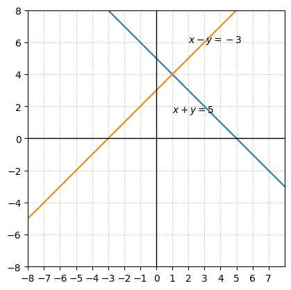
The system of linear equations below is consistent and independent with one solution.
The lines intersect at (1,4).
x = np.linspace(-100,100)

fig, ax = plt.subplots()
ax.plot(x,(5-x))
ax.plot(x,(3+x))

ax.text(1,1.6,'$x+y = 5$')
ax.text(2,6,'$x-y = -3$')

ax.set_xlim(-8,8)
ax.set_ylim(-8,8)
ax.axvline(color='k',linewidth = 1)
ax.axhline(color='k',linewidth = 1)

ax.set_xticks(list(range(-8,8)))
ax.set_aspect('equal')
ax.grid(True,ls=':')
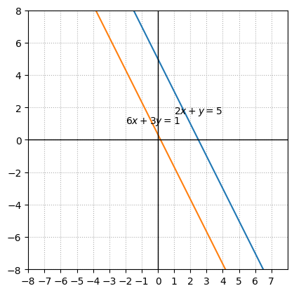
The system of linear equations below is consistent and independent with one solution.
The system is inconsistent because they have the same slopes but different intercepts. Equation 1 can be written as \(y = -2x + 5\) and equation 2 can be written as \(y = -2x + \frac{1}{3}\).
x = np.linspace(-100,100)

fig, ax = plt.subplots()
ax.plot(x,(-2*x + 5))
ax.plot(x,(-2*x + (1/3)))

ax.text(1,1.6,'$2x+y = 5$')
ax.text(-2,1,'$6x+3y = 1$')

ax.set_xlim(-8,8)
ax.set_ylim(-8,8)
ax.axvline(color='k',linewidth = 1)
ax.axhline(color='k',linewidth = 1)

ax.set_xticks(list(range(-8,8)))
ax.set_aspect('equal')
ax.grid(True,ls=':')
Solving system of equations using inverses and matrices#
To solve a system of n equations with n unknowns using an n × n matrix and its inverse, do the following:
Write each of the equations in the system with the variables in the same order and the constant on the other side of the equal sign from the variables.
Construct a coefficient matrix (a square matrix whose elements are the coefficients of the variables).
Write the constant matrix (an n × 1 column matrix) using the constants in the equations.
Find the inverse of the coefficient matrix.
Multiply the inverse of the coefficient matrix times the constant matrix.
The resulting matrix shows the values of the variables in the solution of the system.
For example, to solve the system of equations:
Constructing a coefficient matrix using 0s for the missing variables.
A = np.matrix(np.array([-1,-1,-1,4,5,0,0,1,-3]).reshape(3,3))
print("A = \n", A)
A =
 [[-1 -1 -1]
 [ 4  5  0]
 [ 0  1 -3]]
Writing the constant matrix.
B = np.array([3,-6,5]).reshape(-1,1)
print("B = \n", B)
B =
 [[ 3]
 [-6]
 [ 5]]
Finding the inverse of the coefficient matrix.
Ainv = inv(A)
print("A^-1 = \n", Ainv)
A^-1 =
 [[ 15.   4.  -5.]
 [-12.  -3.   4.]
 [ -4.  -1.   1.]]
Multiplying the inverse of the coefficient matrix times the constant matrix.
sol = Ainv @ B
print("Solution =\n", sol)
Solution =
 [[-4.]
 [ 2.]
 [-1.]]
# Alternatively you can use numpy linalg solve
np.linalg.solve(A,B)
array([[-4.],
       [ 2.],
       [-1.]])
Augmented matrix#
Not all matrices have inverses. Some square matrices are non-singular.
Linear combination of Vectors#
Using both scalar multiplication and matrix addition, a linear combination uses vectors in a set to create a new vector that’s the same dimension as the vectors involved in the operations.
A linear combination of vectors is written as \(y = c_1v_1 + c_2v_2 + c_3v_3 + \dots + c_kv_k\) where \(v_1, v_2, v_3, \dots, v_k\) are vectors and \(c_i\) is a real coefficient called a \(scalar\).
Given a set of vectors with the same dimensions, many different linear combinations may be formed. And, given a vector, you can determine if it was formed from a linear combination of a particular set of vectors.
Below are three vectors:
And here is a linear combination \(y = 3\mathbf{v_1} + 4\mathbf{v_2} + 2\mathbf{v_3}\)
v1 = np.array([3,-2,0]).reshape(-1,1)
v2 = np.array([4,0,-4]).reshape(-1,1)
v3 = np.array([8,-1,-3]).reshape(-1,1)

y = 3*v1 + 4*v2 + 2*v3

print("y = \n", y)
y =
 [[ 41]
 [ -8]
 [-22]]
The final result is another \(3 \times 1\) vector.
If you have no restrictions on the values of the scalars, then you have an infinite number of possibilities for the resulting vectors. What you want to determine, though, is whether a particular vector is the result of some particular linear combination of a given set of vectors.
You do this by solving for the individual scalars that produce the vector. Using the vectors \(v_1\) , \(v_2\), and \(v_3\), you write the equation \(x_1v_1+ x_2v_2 + x_3v_3 = b\), where \(x_i\) is a scalar and \(b\) is the target vector.
Multiplying each vector with its respective scalar,
You can write this as a system of linear equatrions.
Now, create an augmented matrix and perform row operations to produce a reduced row echelon form as explained in the previous section.
We can represent the system of linear equations as a matrix and the resultant vector as the outputnand use numpy.linalg.solve to find the solution. The solutions correspond to the scalars needed for the vector equation \(x_1v_1 + x_2v_2 + x_3v_3 = b\).
V = np.matrix(np.concatenate([v1,v2,v3], axis = 1))
v_out = np.array([4,5,-1]).reshape(-1,1)

s = np.linalg.solve(V,v_out)

print("Linear equations represented as a matrix V = \n", V)
print("Output vector b = \n", v_out)
print("Scalars needed for the vector equation x1,x2,x3= \n", s)
Linear equations represented as a matrix V =
 [[ 3  4  8]
 [-2  0 -1]
 [ 0 -4 -3]]
Output vector b =
 [[ 4]
 [ 5]
 [-1]]
Scalars needed for the vector equation x1,x2,x3=
 [[-4.]
 [-2.]
 [ 3.]]
Visualizing linear combination of vectors#
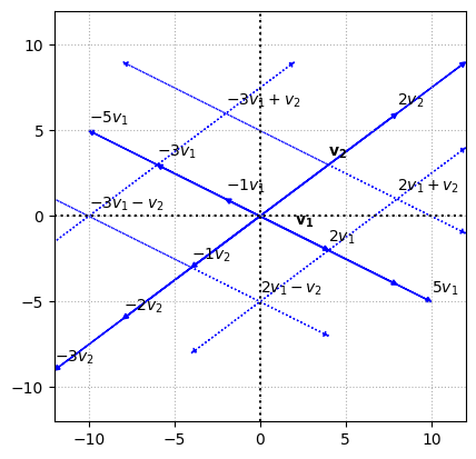
Lets say we want to represent a \(2 \times 1\) vector in the coordinate system. The vectors
Suppose the linear combinations of vectors are \(-3\mathbf{v_1}-\mathbf{v_2}, -3\mathbf{v_1}+\mathbf{v_2}, 2\mathbf{v_1}-\mathbf{v_2}, 2\mathbf{v_1}+\mathbf{v_2}\), then the linear combinations of vectors are represented using parallel lines drawn through the multiples of the points representing the vectors.
Show code cell source
fig, ax = plt.subplots()
options = {"head_width":0.3, "head_length":0.3, "length_includes_head":True}

v1 = np.array([2,-1]).reshape(-1,1)
v2 = np.array([4,3]).reshape(-1,1)

# plot the actual vectors
ax.arrow(0,0,v1[0][0] * 4,v1[1][0] * 4,fc='b',ec='b',**options)
ax.text(v1[0][0],v1[1][0] + .5,'$\mathbf{v_1}$')
ax.arrow(0,0,v2[0][0] * 3,v2[1][0] * 3,fc='b',ec='b',**options)
ax.text(v2[0][0],v2[1][0] + .5,'$\mathbf{v_2}$')

# plot the scaled vectors
for s in [-5,-3,-1,2,5]:
    v1_s = s * v1
    ax.arrow(0,0,v1_s[0][0],v1_s[1][0],fc='b',ec='b',**options)
    ax.text(v1_s[0][0],v1_s[1][0] + .5,f'${s}v_1$')

for s in [-2,-3,-1,2]:
    v2_s = s * v2
    ax.arrow(0,0,v2_s[0][0],v2_s[1][0],fc='b',ec='b',**options)
    ax.text(v2_s[0][0],v2_s[1][0] + .5,f'${s}v_2$')

# add dashed line
options = {"head_width":0.3, "head_length":0.3, "length_includes_head":True, "linestyle" : ':'}

# -3v1 - v2
v1_s = -3 * v1
v2_s = -1 * v2
ax.arrow(v1_s[0][0],v1_s[1][0],v2_s[0][0] * 2,v2_s[1][0] * 2,fc='b',ec='b',**options)
ax.arrow(v2_s[0][0],v2_s[1][0],v1_s[0][0] * 2,v1_s[1][0] * 2,fc='b',ec='b',**options)
v_n = v1_s + v2_s
ax.text(v_n[0][0],v_n[1][0] + .5,'$-3v_1 - v_2$')

# -3v1 + v2
v1_s = -3 * v1
ax.arrow(v1_s[0][0],v1_s[1][0],v2[0][0] * 2,v2[1][0] * 2,fc='b',ec='b',**options)
ax.arrow(v2[0][0],v2[1][0],v1_s[0][0] * 2,v1_s[1][0] * 2,fc='b',ec='b',**options)
v_n = v1_s + v2
ax.text(v_n[0][0],v_n[1][0] + .5,'$-3v_1 + v_2$')

# 2v1 - v2
v1_s = 2 * v1
v2_s = -1 * v2
ax.arrow(v1_s[0][0],v1_s[1][0],v2_s[0][0] * 2,v2_s[1][0] * 2,fc='b',ec='b',**options)
ax.arrow(v2_s[0][0],v2_s[1][0],v1_s[0][0] * 2,v1_s[1][0] * 2,fc='b',ec='b',**options)
v_n = v1_s + v2_s
ax.text(v_n[0][0],v_n[1][0] + .5,'$2v_1 - v_2$')

# 2v1 + v2
v1_s = 2 * v1
ax.arrow(v1_s[0][0],v1_s[1][0],v2[0][0] * 2,v2[1][0] * 2,fc='b',ec='b',**options)
ax.arrow(v2[0][0],v2[1][0],v1_s[0][0] * 2,v1_s[1][0] * 2,fc='b',ec='b',**options)
v_n = v1_s + v2
ax.text(v_n[0][0],v_n[1][0] + .5,'$2v_1 + v_2$')

# settings
ax.set_aspect('equal')
ax.grid(True,ls=':')
ax.axvline(x=0,color="k",ls=":")
ax.axhline(y=0,color="k",ls=":")
ax.grid(True)
ax.axis([-12,12,-12,12])
ax.set_aspect('equal')
Span of a set of vectors#
The set of all linear combinations of a set of vectors \(\{v_1, v_2, \dots, v_n \}\) is called its span. Each vector in the \(span\{v_1, v_2, \dots, v_n \}\) is of the form \(c_1v_1 + c_2v_2 + \dots + c_nv_n\) where \(c_i\) is a real number scalar.
Replacing the scalars with real numbers, you produce new vectors of the same dimension. With all the real number possibilities for the scalars, the resulting set of vectors is infinite.
Determining whether a particular vector belongs in the span#
To determine whether a vector is part of a span, you need to determine which linear combination of the vectors produces that target vector.
Consider a vector set \(\{\mathbf{v_1}, \mathbf{v_2}, \mathbf{v_3}\}\) where
To determine if the vector $\( \mathbf{b} = \begin{bmatrix} -11 \\ -13 \\ 6\end{bmatrix} \)\( belongs to the \)span{\mathbf{v_1}, \mathbf{v_2}, \mathbf{v_3}}$, we need to find the solution for the vector equation
which is a system of linear equations.
v1 = np.array([1,-2,0]).reshape(-1,1)
v2 = np.array([4,2,-1]).reshape(-1,1)
v3 = np.array([3,-1,2]).reshape(-1,1)

V = np.matrix(np.concatenate([v1,v2,v3],axis = 1))
b = np.array([-11,-13,6]).reshape(-1,1)

print("c1, c2, c3 = \n", np.linalg.solve(V,b))
c1, c2, c3 =
 [[ 2.]
 [-4.]
 [ 1.]]
The linear combination of the vectors does produce the target vector. The vector \(\mathbf{b}\) does belong in the span.
Ax = b#
If \(A\) is an \(m \times n\) matrix whose columns are designated by \(a_1, a_2 , \dots, a_n\) and if vector \(x\) has \(n\) rows, then the multiplication \(A\mathbf{x}\) is equivalent to having each of the elements in vector \(x\) times one of the columns in matrix \(A\). We are rewriting the multiplication problem as a linear combination.
B = np.array([2,3,1,0,-1,4,1,-3]).reshape(2,4)
z = np.array([1,-3,2,2]).reshape(-1,1)

Bz = B @ z

print("B = \n", B)
print("z = \n", z)
print("B * z = \n", Bz)
B =
 [[ 2  3  1  0]
 [-1  4  1 -3]]
z =
 [[ 1]
 [-3]
 [ 2]
 [ 2]]
B * z =
 [[ -5]
 [-17]]
j = np.array([])
# create a for loop with iterations equal to the number of columns in the matrix
for i in range(B.shape[1]):
    # for each iteration subset the matrix with the ith col and ith row for the vector
    Bz_i = z[i] * B[:,i]
    # append the scalar and col product to an array
    j = np.append(j,[Bz_i])
j = j.reshape(-1,B.shape[0])
Bz = np.sum(j, axis = 0).reshape(-1,1)
print(Bz)
[[ -5.]
 [-17.]]
The following properties apply to the products of matrices and vectors. If \(A\) is an \(m \times n\) matrix, \(u\) and \(v\) are \(n \times 1\) vectors, and \(c\) is a scalar, then:
This is the commutative property of scalar multiplication.
This is the distributive property of scalar multiplication.
Unique solution#
The equation \(A\mathbf{x} = \mathbf{b}\) has a solution only when \(\mathbf{b}\) is a linear combination of the columns of matrix \(A\). Also, \(\mathbf{b}\) is in the span of \(A\) when there is a solution to \(A\mathbf{x} = \mathbf{b}\).
To determine whether you have a solution, use the tried-and-true method of creating an augmented matrix corresponding to the columns of \(A\) and the vector \mathbf{b} and then performing row operations.
Given a matrix \(A\) and a vector \(\mathbf{b}\), find the vector x that solves the equation.
So the matrix equation \(A\mathbf{x} = \mathbf{b}\) is
and the augmented matrix is
Now, performing row operations, we change the matrix to reduced echelon form to determine the solution — what each \(x_i\) represents.
# alternatively we can directly generate the rref using sympy package
# import sympy
from sympy import *

# create the augmented matrix
A_aug = Matrix([[1,-2,2,1,2], [1,-1,5,0,10], [2,-2,11,2,20], [0,2,8,1,17]])
print("Augmented matrix A =")
display(A_aug)

# Use sympy.rref() method
A_rref = A_aug.rref()

print("The Reduced Row echelon form of matrix A and the pivot columns : {}".format(A_rref))
Augmented matrix A =
The Reduced Row echelon form of matrix A and the pivot columns : (Matrix([
[1, 0, 0, 0,  1],
[0, 1, 0, 0,  1],
[0, 0, 1, 0,  2],
[0, 0, 0, 1, -1]]), (0, 1, 2, 3))
The pivot columns or tuple represent the columns that constitute the reduced row echelon form and the last column has the elements of the vector \(x_i\).
In the RREF (reduced row echelon form) matrix, we see that there is a leading 1 in every column that corresponds to a variable, the system has a unique solution. In RREF, the leading entry in each row is 1, the leading 1 in each row occurs to the right of the leading 1 in the previous row, and each column containing a 1 has zeros everywhere else.
Multiple solutions#
Consider a matrix \(A\) and a vector \(\mathbf{b}\) in the equation \(A\mathbf{x} = \mathbf{b}\), and its augmented matrix to be
# create the augmented matrix
A_aug = Matrix([[1,3,1,6], [3,-2,-8,7], [4,5,-3,17]])
print("Augmented matrix A =")
display(A_aug)
# Use sympy.rref() method
A_rref = A_aug.rref()

print("The Row echelon form of matrix A and the pivot columns : {}".format(A_rref))
Augmented matrix A =
The Row echelon form of matrix A and the pivot columns : (Matrix([
[1, 0, -2, 3],
[0, 1,  1, 1],
[0, 0,  0, 0]]), (0, 1))
The last row in the augmented matrix contains all \(0s\). Having a row of \(0s\) indicates that you have more than one solution for the equation.
To proceed further, take the reduced form of the matrix and go back to a system of equations format, with the reduced matrix multiplying vector \(\mathbf{x}\) and setting the product equal to the last column.
Do the matrix multiplication and right the corresponding equations
Replace \(x_3\) with a parameter \(k\). Then the corresponding equations are $\(x_3 = k\)\( \)\(x_2 = 1 - k\)\( \)\(x_1 = 3 + 2k\)$
The vector \(\mathbf{b}\) can be written as
where \(k\) is any real number. Substituting a value for k provides the solution.
No solution#
# create the augmented matrix
A_aug = Matrix([[2,-1,1,1], [1,1,-1,2], [3,-1,1,0]])
print("Augmented matrix A =")
display(A_aug)
# Use sympy.rref() method
A_rref = A_aug.rref()

print("The Row echelon form of matrix A and the pivot columns : {}".format(A_rref))
Augmented matrix A =
The Row echelon form of matrix A and the pivot columns : (Matrix([
[1, 0,  0, 0],
[0, 1, -1, 0],
[0, 0,  0, 1]]), (0, 1, 3))
The last row in the matrix has three \(0s\) and then a number. Translating this into an equation, you have \(0x1 + 0x2 + 0x3 = 1\). The statement is impossible. When you multiply by 0, you always get a 0, not some other number. So the matrix-vector equation has no solution.
Homogeneous systems#
A system of linear equations is said to be homogeneous if it is of the form:
where each \(x_i\) is a variable and each \(a_{ij}\) is a real-number coefficient. Each sum of coefficient-variable multiples is set equal to 0 i.e. \(A\mathbf{x} = 0\).
Unlike a general system of linear equations, a homogeneous system of linear equations always has at least one solution — a solution is guaranteed.The guaranteed solution occurs when you let each variable be equal to 0. The solution where everything is 0 is called the trivial solution.
If a homogeneous system of linear equations has fewer equations than it has unknowns, then it has a nontrivial solution. Further, a homogeneous system of linear equations has a nontrivial solution if and only if the system has at least one free variable. A free variable (also called a parameter) is a variable that can be randomly assigned some numerical value. The other variables are then related to the free variable through some algebraic rules.
To understand if a homogeneous system of equations has non-trivial solution or a trivial solution, we can follow a procedure. We can represent the equations in the augmented matrix form and perform row operations to get the reduced row echelon form. Then we follow the general rules that apply to this form. If all the values in the last row are \(0s\), then the system has non-trivial solutions.
Linear independence#
The vectors \({v_1, v_2, \dots, v_n}\) are linearly independent if the equation involving linear combinations, \(a_1v_1 + a_2v_2 + \dots + a_nv_n = 0\), is true only when the scalars \((a_i)\) are all equal to 0. The vectors are linearly dependent if the equation has a solution when at least one of the scalars is not equal to 0.
In general, if one of the vectors is a linear combination of the other vectors, then the vectors are linearly dependent.
To test under what circumstances the equation \(a_1v_1 + a_2v_2 + a_3v_3=0\), write out the equation with the vectors.
Then create the augmented matrix and perform row operations.
# create the augmented matrix
A_aug = Matrix([[1,4,3,0], [-2,0,-1,0], [0,8,5,0]])
print("Augmented matrix A =")
display(A_aug)
# Use sympy.rref() method
A_rref = A_aug.rref()

print("The Row echelon form of matrix A and the pivot columns : {}".format(A_rref))
Augmented matrix A =
The Row echelon form of matrix A and the pivot columns : (Matrix([
[1, 0, 1/2, 0],
[0, 1, 5/8, 0],
[0, 0,   0, 0]]), (0, 1))
The bottom row has all \(0s\). The set of vectors is linearly dependent. The requirement for linear dependence is that you have more than just the trivial solution.
You can rewrite the above reduced matrix as by letting \(a_3 = k\).
Then
by substituting for \(k\), one can find the solutions.
For a given set of vectors, if the augmented matrix after performing row operations looks like an identity matrix, then the vectors are linearly independent i.e. \(a_1 = a_2 = a_3 = 0\).
# create the augmented matrix
A_aug = Matrix([[1,0,2,0], [2,1,0,0], [1,1,1,0], [4,1,7,0]])
print("Augmented matrix A =")
display(A_aug)
# Use sympy.rref() method
A_rref = A_aug.rref()

print("The Row echelon form of matrix A and the pivot columns : {}".format(A_rref))
Augmented matrix A =
The Row echelon form of matrix A and the pivot columns : (Matrix([
[1, 0, 0, 0],
[0, 1, 0, 0],
[0, 0, 1, 0],
[0, 0, 0, 0]]), (0, 1, 2))
Shortcuts to find Linear dependency:
A set containing only one vector is linearly independent if that one vector is not the zero vector.
A set containing two vectors is linearly independent as long as one of the vectors is not a multiple of the other vector.
A set containing n × 1 vectors has linearly dependent vectors if the number of vectors in the set is greater than n.
A set containing the zero vector is always linearly dependent. (the zero vector is a multiple of any other vector in the set — it’s another vector times the scalar 0).
If vectors are linearly independent, then removing an arbitrary vector, \(\mathbf{v_i}\), does not affect the linear independence.
If the set of vectors \({\mathbf{v_1}, \mathbf{v_2}, \dots, \mathbf{v_n}}\) contains all distinct (different) unit vectors (has one element that’s a \(1\)), then that set has linear independence
Basis#
A set of vectors \({\mathbf{v_1}, \mathbf{v_2}, \dots, \mathbf{v_n}}\) is said to form a basis for a vector space if both of the following are true:
The vectors \(\mathbf{v_1}, \mathbf{v_2}, \dots, \mathbf{v_n}\) span the vector space.
The vectors \(\mathbf{v_1}, \mathbf{v_2}, \dots, \mathbf{v_n}\) are linearly independent
In simpler words, a set of vectors that can be used to represent any vector in the space through linear combinations.
Natural basis or Standard basis#
For all the \(3 \times 1\) vectors, the set of 3 unit vectors is the basis. They are also other set of vectors that can be used to form the basis of \(\mathbb{R}^3\). For example
Using this set, you can write any possible \(3 \times 1\) vector as a linear combination of the vectors in this set. It is possible to have more than one basis for a vector space. Below you will see how we can get the date of landing on the moon by the Apollo 11 crew using the set of vectors.
The dimension of a vector space is the number of vectors in the basis of the vector space. So the dimension for above basis is 3.
# create the augmented matrix
A_aug = Matrix([[1,0,1,7], [1,1,2,20], [1,0,3,1969]])
print("Augmented matrix A =")
display(A_aug)
# Use sympy.rref() method
A_rref = A_aug.rref()

print("The Row echelon form of matrix A and the pivot columns : {}".format(A_rref))
Augmented matrix A =
The Row echelon form of matrix A and the pivot columns : (Matrix([
[1, 0, 0, -974],
[0, 1, 0, -968],
[0, 0, 1,  981]]), (0, 1, 2))
Determining a basis#
If you have vectors \(\mathbf{v_1}, \mathbf{v_2}, \dots, \mathbf{v_n}\) , to find vectors which form a basis for the span of the given vectors:
Form the linear combination \(a_1\mathbf{v_1}, a_2\mathbf{v_2}, \dots, a_n\mathbf{v_n}\), where each \(a_i\) is a real number.
Construct the corresponding augmented matrix.
Transform the matrix to reduced row echelon form.
Identify the vectors in the original matrix corresponding to columns in the reduced matrix that contain leading \(1s\) (the first nonzero element in the row is a \(1\)).
# create the augmented matrix
A_aug = Matrix([[1,-1,1,3,0,4,-2,1,0], [2,-1,4,4,1,9,-3,0,0], [1,1,5,-1,2,6,0,-3,0]])
print("Augmented matrix A =")
display(A_aug)
# Use sympy.rref() method
A_rref = A_aug.rref()

print("The Row echelon form of matrix A and the pivot columns : {}".format(A_rref))
Augmented matrix A =
The Row echelon form of matrix A and the pivot columns : (Matrix([
[1, 0, 3,  1, 1, 5, -1, -1, 0],
[0, 1, 2, -2, 1, 1,  1, -2, 0],
[0, 0, 0,  0, 0, 0,  0,  0, 0]]), (0, 1))
Here the first \(2\) vectors have leading \(1's\) in the reduce echelon form. So the basis for the \(8\) vectors is the set of first \(2\) vectors.
If we change the order of the vectors and write the augmented matrix and perform the row operations:
# create the augmented matrix
A_aug = Matrix([[3,1,-1,1,0,4,1,-2,0], [4,2,-1,4,1,9,0,-3,0], [-1,1,1,5,2,6,-3,0,0]])
print("Augmented matrix A =")
display(A_aug)
# Use sympy.rref() method
A_rref = A_aug.rref()

print("The Row echelon form of matrix A and the pivot columns : {}".format(A_rref))
Augmented matrix A =
The Row echelon form of matrix A and the pivot columns : (Matrix([
[1, 0, -1/2, -1, -1/2, -1/2,  1, -1/2, 0],
[0, 1,  1/2,  4,  3/2, 11/2, -2, -1/2, 0],
[0, 0,    0,  0,    0,    0,  0,    0, 0]]), (0, 1))
The first \(2\) columns are still the vectors having leading \(1's\). So the first \(2\) vectors can also be a basis for the span of vectors.
Basis of Polynomials#
A polynomial is a sum of variables and their coefficients where the variables are to raised to whole-number powers. The general format is \(a_nx^n + a_{n-1}x^{n-1} + \dots + a_2x^2 + a_1x^1 + a_0\).the degree of the polynomial is whichever is the highest power of any variable.
The terms in the set \({x^2, x, 1}\) are a span of \(\mathbb{P}^2\), because all second-degree polynomials are the result of some linear combination \(a_2x^2 + a_1x + a_0(1)\).
The elements in the set are linearly independent, because \(a_2x^2 + a_1x + a_0(1)\) is true only in the case of the trivial solution where each coefficient is \(0\). So the elements in the set form a basis for \(\mathbb{P}^2\).
To determine if \(Q = \{x^3 + 3, 2x^2 - x, x + 1, 2\}\) spans \(\mathbb{P}^3\) and if the elements of \(Q\) are linearly independent we shall proceed first by writing them as a linear combination such that
In general, a third-degree polynomial is of the form \(ax^3 + bx^3 + cx +d\). So here
Solving the equations for the values
Now to check if a polynomial \(x^3 + 4x^2 - 5x + 3\) can be written by using the above scalars and the basis, we substitue \(a = 1, b = 4, c = -5, d = 3\).
Linear Transformations#
A linear transformation is a particular type of transformation, where one set of vectors is transformed into another vector set using some linear operator.
Let transformation be denoted as \(T\). Then a linear transformation can be written as
where
Here transformation \(T\) takes in a \(3 \times 1\) vector and transforms it into a \(2 \times 1\) vector.
So \(T(\mathbf{v})\) is
Some properties of linear transformations:
\(T(\mathbf{u} + \mathbf{v}) = T(\mathbf{u}) + T(\mathbf{v})\)
\(T(c\mathbf{v}) = cT(\mathbf{v})\)
In order to check if a transformation is linear, we can use these properties to check if the transformation satisfies these conditions.
Transformation composition#
Transformation composition can be defined as \((T_1T_2)(\mathbf{v}) = T_1(T_2(\mathbf{v}))\)
The associative property states that when you perform transformation composition on the first of two transformations and then the result on a third, you get the same result as performing the composition on the last two transformations and then performing the transformation described by the first on the result of those second two.
For scalar multiplication no matter where you introduce the scalar multiple, the result is the same.
The additive identity transformation \(T_0\) takes a vector and transforms that vector into a zero vector.
The multiplicative identity transformation \(I\) when given a vector \(\mathbf{v}\) is
There are several other properties that could be explored such as tying distribution, scalar multiplication and addition altogether.
Matrix of a Linear Transformation#
One can make use of matrices to apply linear transformations. For example consider a linear transfromation where
Then you can use a \(2 \times 2\) matrix \(A\) such that
So \(T(\mathbf{v}) = A * \mathbf{v}\)
One can get such matrix by writing the transformation as a sum of different vectors of coefficients. For example
Hence the matrix is
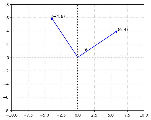
Visualizing transformation involving rotation#
For our convenience, lets stick to vectors in \(\mathbb{R}^2\). To rotate a vector \(\mathbf{v}\) by \(\theta\) degrees about the origin in a counter clockwise direction, the matrix \(A\) use is
To rotate a vector by \(90°\), we can substitute \(\theta\) with \(90\). Since \(\sin90 = 1\) and \(\cos90 = 0\) the resultant matrix is
fig, ax = plt.subplots()
options = {"head_width":0.3, "head_length":0.3, "length_includes_head":True}

v = np.array([6,4]).reshape(-1,1)
A = np.array([0,-1,
              1,0]).reshape(2,2)
Av = A @ v

ax.arrow(0,0,v[0][0],v[1][0],fc='b',ec='b',**options)
ax.arrow(0,0,Av[0][0],Av[1][0],fc='b',ec='b',**options)

ax.text(1,1,'$\mathbf{v}$')
ax.text(v[0][0],v[1][0],'$(6,4)$')
ax.text(Av[0][0],Av[1][0],'$(-4,6)$')

# settings
ax.set_aspect('equal')
ax.grid(True,ls=':')
ax.axvline(x=0,color="k",ls=":")
ax.axhline(y=0,color="k",ls=":")
ax.grid(True)
ax.axis([-10,10,-8,8])
ax.set_aspect('equal')
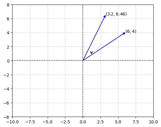
Rotation of the vector by \(30°\)
fig, ax = plt.subplots()
options = {"head_width":0.3, "head_length":0.3, "length_includes_head":True}

v = np.array([6,4]).reshape(-1,1)
# since numpy trig funcs take in radians, we first convert rads to degs
A = np.array([np.cos(np.deg2rad(30)),-np.sin(np.deg2rad(30)),
              np.sin(np.deg2rad(30)),np.cos(np.deg2rad(30))]).reshape(2,2)
Av = A @ v

ax.arrow(0,0,v[0][0],v[1][0],fc='b',ec='b',**options)
ax.arrow(0,0,Av[0][0],Av[1][0],fc='b',ec='b',**options)

ax.text(1,1,'$\mathbf{v}$')
ax.text(v[0][0],v[1][0],'$(6,4)$')
ax.text(Av[0][0],Av[1][0],f'$({np.round(Av[0][0],2)},{np.round(Av[1][0],2)})$')

# settings
ax.set_aspect('equal')
ax.grid(True,ls=':')
ax.axvline(x=0,color="k",ls=":")
ax.axhline(y=0,color="k",ls=":")
ax.grid(True)
ax.axis([-10,10,-8,8])
ax.set_aspect('equal')
Translation, dilation and contraction#
To translate a vector from one point to another point involves performing a transformation that adds a distance vector to the current vector i.e.
This operation can dilate (expand) or contract (shrink) the vector based on the distance vector.
To double the magnitude of a vector, the matrix required for the linear transformation \(D*\mathbf{v}\) is
In general the multiplier is across the diagonal and \(0s\) in all other positions of the matrix. If the multiplier is greater than \(1\) then you have a dilation, if it is between \(0\) and \(1\) you have a contraction.
Kernel and range of a linear transformation#
TBC
Determinants#
Matrix permutation#
A permutation matrix is formed by rearranging the columns of an identity matrix. If \(n\) is the number of rows and columns in the identity matrix, then \(n!\) is the number of permutations.
One way of identifying the different permutation matrices is to use numbers such as \(312\) or \(213\) to indicate where the digit \(1\) is positioned in a particular row. For example, permutation \(312\) is represented by the fourth matrix, because row \(1\) has its \(1\) in the third column, row \(2\) has its \(1\) in the first column, and row \(3\) has its \(1\) in the second column.
from itertools import permutations

identity_mat = np.eye(3)
perm_itr = permutations(identity_mat)
perm_mats = np.array(list(perm_itr))
perm_mats
array([[[1., 0., 0.],
        [0., 1., 0.],
        [0., 0., 1.]],

       [[1., 0., 0.],
        [0., 0., 1.],
        [0., 1., 0.]],

       [[0., 1., 0.],
        [1., 0., 0.],
        [0., 0., 1.]],

       [[0., 1., 0.],
        [0., 0., 1.],
        [1., 0., 0.]],

       [[0., 0., 1.],
        [1., 0., 0.],
        [0., 1., 0.]],

       [[0., 0., 1.],
        [0., 1., 0.],
        [1., 0., 0.]]])
Inverse permutation#
An inverse permutation is a permutation in which each number and the number of the place it occupies are exchanged.
For example, consider the permutation \(25413\). The inverse permutation associated is \(41532\). The way it works is : 1 was in the fourth position, so I put the 4 in the first position; 2 was in the first position, so I put the 1 in the second position; and so on…
When you multiply a matrix and its inverse, the resultant is an identity matrix.
P = np.array([0,1,0,0,0,0,0,0,0,1,0,0,0,1,0,1,0,0,0,0,0,0,1,0,0]).reshape(5,5)
P_inv = np.array([0,0,0,1,0,1,0,0,0,0,0,0,0,0,1,0,0,1,0,0,0,1,0,0,0]).reshape(5,5)

print('Permutation Matrix 25413 : \n', P)
print('Permutation Matrix 41532 : \n', P_inv)
print('P x P_inv : \n', P @ P_inv)
Permutation Matrix 25413 :
 [[0 1 0 0 0]
 [0 0 0 0 1]
 [0 0 0 1 0]
 [1 0 0 0 0]
 [0 0 1 0 0]]
Permutation Matrix 41532 :
 [[0 0 0 1 0]
 [1 0 0 0 0]
 [0 0 0 0 1]
 [0 0 1 0 0]
 [0 1 0 0 0]]
P x P_inv :
 [[1 0 0 0 0]
 [0 1 0 0 0]
 [0 0 1 0 0]
 [0 0 0 1 0]
 [0 0 0 0 1]]